Machine Learning Time Series Techniques for Accurate Predictions and Forecasting

Time is a precious resource that governs our lives, and possessing a reliable method for predicting and forecasting future events has always been a human aspiration. In the digital age, we have a wealth of information at our disposal, particularly in the form of time series data.

This conception means any data that is sampled and organized based on a time scale dimension: days, months, years, and so on. It is expected to hold valuable insights that can help us make informed decisions and shape business strategies and move in alignment with anticipated future events and trends. Time series data examples include:

1. Financial markets: stock prices, exchange rates, and trading volumes.
2. Climate and weather: temperature, rainfall, and wind speed.
3. Sales and demand forecasting: product sales data over time.
4. Website traffic and user behavior: page views, click-through rates, and conversion rates.
5. Energy consumption: electricity usage and energy demand.
6. Sensor data: measurements from sensors in manufacturing, healthcare, and transportation.
7. Social media activity: likes, comments, shares, and follower counts.

These examples demonstrate the diverse presence of time series data in strategic fields of business data analytics, such as finance, weather, sales, online analytics, energy management, sensor monitoring, and social media analysis. Mastering time series machine learning (ML) in each of these domains can yield significant benefits in terms of event forecasting and effective management of factors influencing trends, patterns, and other fluctuations.

In this article, we will embark on a journey to master the art of time series analysis and forecasting using machine learning techniques. Otherwise, if you require immediate help with machine learning for forecasting time series, we recommend that you contact our data engineers for professional assistance. Our team possesses a sophisticated vision and skills for time-series feature engineering and implementation.

Automated Analysis and Forecasting in Time Series Data: Features and Challenges

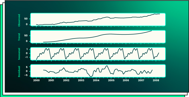
With the advent of machine learning forecasting, we now have powerful tools to analyze and uncover patterns in time series data. This enables us to make accurate predictions and forecasts. Let’s learn about the major data series components:

• Trend. In time series data theory, a trend refers to the varying behavior of values over time. It can be positive (indicating an increasing trend) or negative (indicating a decreasing trend.)
• Seasonality. Seasonality is a characteristic of time-series data that exhibits recurring patterns at regular intervals. These patterns repeat with a constant frequency.
• Remainder. After extracting the trend and seasonality components from the data, what remains is known as the remainder or residual. This represents the portion of the data that does not conform to the trend or the seasonal patterns. The analysis of this remainder can be helpful in detecting anomalies or unexpected fluctuations in the time series.
• Cycle. When a time series displays recurring patterns or fluctuations without a fixed period or seasonality, it is referred to as cyclical behavior. Unlike seasonality, these cycles do not follow a specific and predictable frequency. They may occur due to external factors or underlying patterns that are not easily captured by trend or seasonality components.
• Stationarity. A time series is considered stationary when its statistical properties remain constant over time. This means that the mean, standard deviation, and covariance of the data do not change with time. Stationary time series are easier to analyze and model as their behavior remains consistent.

Time-series data analysis follows a distinct framework compared to static data analysis. As outlined in the previous section, the analysis of time-series data begins by addressing fundamental questions such as:

1. Does the data exhibit a trend?
2. Are there discernible patterns or seasonality in the data?
3. Is the data characterized as stationary or non-stationary?

Key questions in time-series analysis include identifying trends, patterns/seasonality and determining stationarity. In static data analysis, procedures like descriptive, predictive, and prescriptive analytics are common. These procedures are applicable to both time-series and static machine-learning applications. However, certain metrics, such as correlation, are utilized differently within the descriptive, predictive, and prescriptive frameworks. By the way, both types of data can be processed with the help of automated ML.

Time series data is unique in its structure and poses specific challenges for analysis and forecasting:

• Unlike static data, time series data is inherently dynamic and possesses an inherent order based on the time dimension.
• The temporal aspect adds complexity, as the values in the series are dependent on past observations and exhibit trends, seasonality, and irregularities.
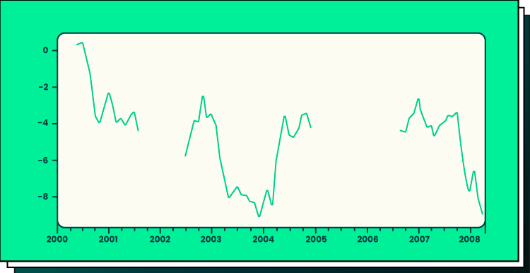
• In the context of time series data, missing values manifest as gaps within the temporal sequence. These gaps represent periods where data observations are absent or incomplete.

As depicted in the graph, there may be conspicuous gaps in the data that defy logical filling through standard imputation strategies typically used with static data. These gaps persist as distinct voids within the dataset, posing a challenge to conventional approaches for handling missing values.

To effectively analyze time series data, it is crucial to comprehend its components, like trends and seasonality. Additionally, time series data may exhibit irregular fluctuations and noise that need to be accounted for during analysis.

Popular Machine Learning Time Series Algorithms: Pros and Cons

Machine learning time series algorithms offer powerful tools to unlock the potential of time series data. These mechanisms enable time series analysis and forecasting, each has its strengths and limitations. Understanding these can help choose the right algorithm for the task at hand. Let’s explore some popular algorithms and their pros and cons:

ARIMA (Autoregressive Integrated Moving Average)

ARIMA is a powerful algorithm widely used in time series analysis. It combines three main components:

• Autoregressive (AR)
• Moving average (MA)
• Time series differencing.

The autoregressive component captures the linear relationship between an observation and a certain number of lagged observations. The moving average component considers the weighted average of past forecast errors. The differencing component helps transform non-stationary data into stationary data by taking the difference between consecutive observations. By combining these components, ARIMA effectively captures trends, seasonality, and noise in time series data.

Let’s consider an example of banking and finance data forecasting. To predict a company’s stock price using the ARIMA model, you begin by obtaining the publicly available stock price data for the past ten years. Once you have this data, you can proceed to train the ARIMA model. In order to determine the appropriate parameters for the ARIMA model, you analyze the data for trends. This involves selecting the order of time series differencing (d) needed to make the data stationary. By examining the autocorrelations and partial autocorrelations, you can then identify the order of regression (p) and the order of moving average (q) for the model.

To choose the best-fitting model, you can utilize various performance metrics such as the Akaike Information Criterion (AIC), Bayesian Information Criterion (BIC), maximum likelihood, and standard error. These metrics help assess the model’s goodness of fit and ensure that it captures the important features and patterns within the stock price data. By systematically analyzing the data and selecting the optimal parameters, the ARIMA model can provide valuable insights and predictions regarding the company’s stock price. This approach allows you to leverage historical trends and patterns to make informed decisions and forecasts in the financial domain.

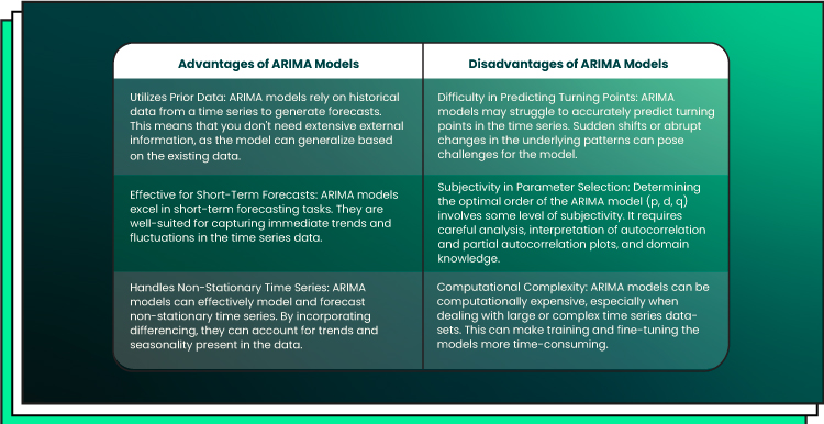
Conclusion: ARIMA, with its simplicity and interpretability, is suitable for shorter-term forecasts and works well with stationary data. However, it may struggle with complex patterns and long-term dependencies.

LSTM (Long Short-Term Memory)

LSTM is a type of recurrent neural network (RNN) that excels in modeling sequences and time dependencies. Unlike traditional feedforward neural networks, LSTM networks have a unique memory cell structure that enables them to retain and utilize information over longer time periods. This makes LSTM particularly effective in capturing long-term dependencies in time series data. LSTM models can learn complex patterns and relationships within the data, making them suitable for deep learning time series in the fields like:

• Speech recognition
• Natural language processing
• Stock market prediction.

The network’s ability to selectively forget or remember information allows it to handle non-stationary time series data and capture temporal dependencies across different time scales.

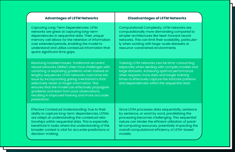
Conclusion: LSTM shines when handling non-linear patterns and long-term dependencies. Its ability to learn from historical data makes it a formidable choice. Yet, it requires more computational resources and larger datasets for training.

Prophet

Developed by Facebook, Prophet is a robust algorithm specifically designed for time series forecasting. It utilizes an additive model that captures non-linear trends, yearly, weekly, and daily seasonality, as well as holiday effects. It performs exceptionally well when applied to time series data with prominent seasonal patterns and a substantial historical record. One of Prophet’s notable strengths is its ability to handle missing data and adapt to shifts in trends, while also demonstrating robustness in handling outliers.

Prophet proves to be particularly valuable for datasets that exhibit the following characteristics:

• Encompass a substantial time span, spanning months or years, with granular and detailed historical observations captured at an hourly, daily, or weekly frequency.
• Display multiple prominent seasonal patterns that occur simultaneously.
• Incorporate significant irregular events that are already known in advance.
• Contain missing data points or notable outliers.
• Showcase non-linear growth trends that are approaching a saturation point.

The growth function serves as a model for capturing the underlying trend of the data. This concept aligns with the familiar linear and logistic functions commonly known to those with basic mathematical knowledge. However, Facebook Prophet introduces a novel concept that allows the growth trend to be flexible and adapt to specific points in the data, known as “changepoints.”

Changepoints represent moments within the data where a noticeable shift in direction occurs.

These points mark transitions where the growth pattern undergoes a change, enabling Prophet to effectively capture and accommodate variations in the trend over time. Prophet operates as an additive regression model that encompasses a piecewise linear or logistic growth curve trend. It incorporates a yearly seasonal component modeled using the Fourier series and a weekly seasonal component modeled using dummy variables. By leveraging these features, Prophet effectively captures the complexities inherent in the aforementioned dataset characteristics.

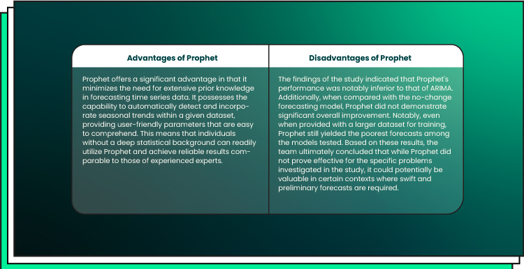
Conclusion: Prophet, with its focus on business forecasting, handles seasonality and holiday effects effectively. However, it may not capture complex interactions and may require careful feature engineering.

Practical Tips for Achieving Accurate Predictions

To harness the power of time series machine learning for forecasting, consider the following practical tips:

Preprocessing the data

Cleanse the data, handle missing values, and address outliers. Apply techniques such as normalization or differencing to achieve stationarity if required.

Time-series feature engineering

Extract meaningful features that capture the underlying patterns in the data. Consider lagged variables, rolling statistics, or Fourier transformations to capture seasonality.

Choosing the right Model

Gain insight into the capabilities and constraints of various algorithms and carefully choose the one that best suits your unique time series. Strike a balance between interpretability and complexity to find the optimal solution.

Separating training and testing

Divide your data into distinct training and testing sets, ensuring that the test set represents unseen future data. Assess your model’s performance by evaluating its predictions on the test set.

Fine-tuning hyperparameters

Refine the hyperparameters of your selected algorithm through techniques such as grid search or Bayesian optimization. This iterative process helps optimize your model’s performance by finding the best combination of settings.

Ensembling

Enhance accuracy and mitigate bias by combining the predictions of multiple models. Ensembling leverages the strengths of individual models to create a more robust and reliable forecasting solution.

Real-World Examples of Time Series Analysis and Forecasting

Energy consumption prediction

Time series deep learning models can predict energy consumption patterns, enabling energy providers to optimize their supply and demand management, reduce costs, and improve sustainability according to numerous factors like expected weather, season, population change, and more.

Stock market forecasting

Traders and investors can tap into the power of deep learning time series algorithms to analyze complex stock market data, accurately forecast trends, uncover potential opportunities for profitable trades, and effectively manage risk. By leveraging advanced techniques such as recurrent neural networks and long short-term memory models, these algorithms can capture intricate patterns and dependencies in the market, providing valuable insights for making informed investment decisions.

Demand forecasting in retail

ML techniques can be applied to analyze historical sales data and predict future demand for various products in the retail industry. This helps retailers optimize their inventory management, ensure product availability, and minimize overstocking or stockouts, leading to improved customer satisfaction and increased profitability.

Conclusion

Machine learning unlocks the hidden gems in time series data. Understanding the unique challenges and selecting suitable algorithms enables accurate predictions. Through careful data preprocessing, feature engineering, model selection, and performance evaluation, we leverage the power of machine learning to master time.

As we refine and advance these AI/ML methods, time series analysis grows even more potent. Contact the Forbytes team to discuss your project and implement time series deep learning and analytics software together.